CSC 53439 EP
Lecture 2
Exploration and Distributional Methods in RL
October 3, 2025
Outline
Part 1
Exploration and Uncertainty
Exploration-Exploitation Dilemma

(Image source: UC Berkeley AI course slide, lecture 11.)
- Agent must explore to discover rewarding actions and states.
- Agent must exploit known information to maximize reward.
- Balancing exploration and exploitation is critical for efficient learning.
- Too much exploration: slow progress; too much exploitation: suboptimal policies.
Unstructured Exploration
$\varepsilon$-greedy
$\quad$ $\mathbf{s} \leftarrow \text{env.reset}()$
$\quad$ DO
$\quad\quad$ $\mathbf{a} \leftarrow \color{red}{\epsilon\text{-greedy}(\mathbf{s}, \hat{Q}_{\mathbf{\omega_1}})}$
$\quad\quad$ $r, \mathbf{s'} \leftarrow \text{env.step}(\mathbf{a})$
$\quad\quad$ Store transition $(\mathbf{s}, \mathbf{a}, r, \mathbf{s'})$ in $\mathcal{D}$
$\quad\quad$ If $\mathcal{D}$ contains "enough" transitions
$\quad\quad\quad$ Sample random batch of transitions $(\mathbf{s}_j, \mathbf{a}_j, r_j, \mathbf{s'}_j)$ from $\mathcal{D}$ with $j=1$ to $m$
$\quad\quad\quad$ For each $j$, set $y_j = \begin{cases} r_j & \text{for terminal } \mathbf{s'}_j\\ r_j + \gamma \max_{\mathbf{a}^\star} \hat{Q}_{\mathbf{\omega_{2}}} (\mathbf{s'}_j)_{\mathbf{a}^\star} & \text{for non-terminal } \mathbf{s'}_j \end{cases}$
$\quad\quad\quad$ Perform a gradient descent step on $\left( y_j - \hat{Q}_{\mathbf{\omega_1}}(\mathbf{s}_j)_{\mathbf{a}_j} \right)^2$ with respect to the weights $\mathbf{\omega_1}$
$\quad\quad\quad$ Every $\tau$ steps reset $\hat{Q}_{\mathbf{\omega_2}}$ to $\hat{Q}_{\mathbf{\omega_1}}$, i.e., set $\mathbf{\omega_2} \leftarrow \mathbf{\omega_1}$
$\quad\quad$ $\mathbf{s} \leftarrow \mathbf{s'}$
$\quad$ UNTIL $\mathbf{s}$ is final
RETURN $\mathbf{\omega_1}$
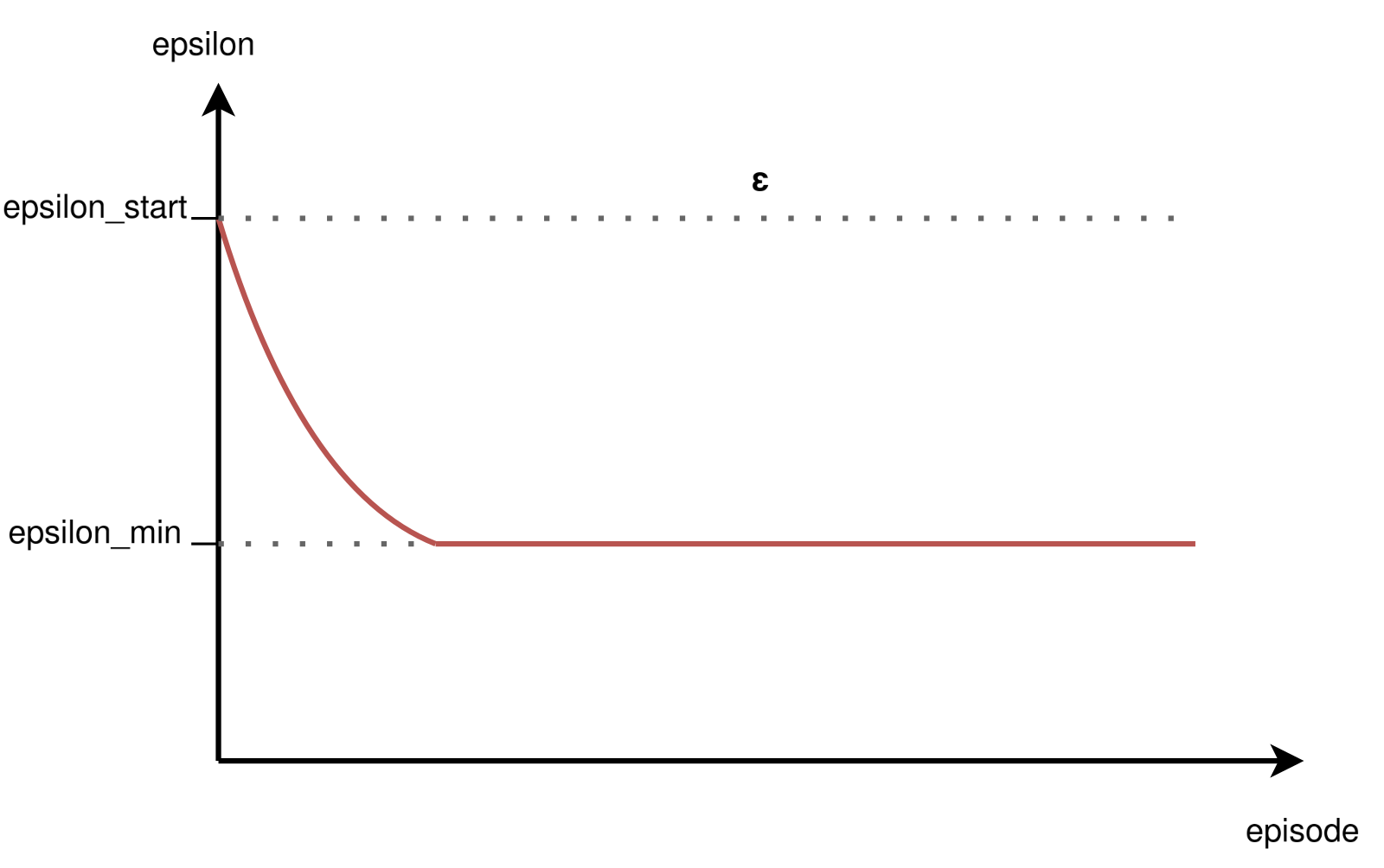
At each step,:
- with probability ε, select a random action;
- with probability 1-ε, select the action with the highest estimated value.
👉 Simple to implement, widely used in discrete action spaces.
Typically, ε is annealed (decreased) over time to shift from exploration to exploitation.
The decay schedule is a hyperparameter and often determined empirically.
Unstructured Exploration
Gaussian Noise
- Add zero-mean Gaussian noise to the action output by the policy.
- Common in algorithms for continuous control (e.g., DDPG, TD3).
- Noise variance can be annealed to reduce exploration over time.
- Encourages smooth, local exploration around the current policy.
$$\mu'(s_t) = \mu(s_t | \theta^{\mu}_t) + \mathcal{N}$$
where $\mu(s_t | \theta^{\mu}_t)$ is the actor network with weights $\theta^{\mu}_t$
and $\mathcal{N}$ is a noise process (e.g. Gaussian or Ornstein-Uhlenbeck).
Limits of Unstructured Exploration
Case Study: Montezuma's Revenge (Atari)
Unstructured methods (ε-greedy, Gaussian noise) struggle in environments with sparse rewards and complex exploration requirements.
Montezuma's Revenge (Atari): classic benchmark for hard exploration.
- Random actions rarely reach rewarding states; agent fails to learn meaningful behavior.
- Motivates the need for intrinsic motivation and structured exploration techniques.
Maximum Entropy RL
Exploration and Robustness via Entropy
Augments the reward with an entropy term to encourage diverse actions: $$ J(\pi) = \mathbb{E}_{\pi} \left[ \sum_t r_t + \alpha \mathcal{H}(\pi(\cdot|s_t)) \right] $$ where $\mathcal{H}$ is the entropy and $\alpha$ controls the exploration-exploitation tradeoff.
- Promotes stochastic policies, improving robustness and exploration.
- Widely used in robotics and continuous action domains.
Maximum Entropy RL
Exploration and Robustness via Entropy
Key algorithms:
-
Soft Q-Learning (SQL): incorporates entropy into Q-learning updates.
Equivalence Between Policy Gradients and Soft Q-Learning, Schulman et al., 2017. -
Soft Actor-Critic (SAC): off-policy actor-critic with entropy maximization,
state-of-the-art for continuous control.
Soft Actor-Critic: Off-Policy Maximum Entropy Deep Reinforcement Learning with a Stochastic Actor, Haarnoja et al., 2018.
Parameter Noise-based Exploration
Noisy Nets, Parameter Space Noise
Intrinsic Reward-based Exploration
Augment environment reward $r_t$ with an intrinsic reward $r^i_t$: $$r_t \leftarrow r_t + \beta \cdot r^i_t$$ where $\beta$ balances exploitation vs exploration.
👉 Encourages agent to explore novel or uncertain states.
Two main approaches:
- Count-based exploration: bonus for visiting rarely seen states.
- Prediction-based exploration: bonus for high prediction error (surprise).
Intrinsic Reward-based Exploration
Count-based Exploration
Assigns exploration bonus inversely proportional to state visit count: $$r^i_t = \frac{1}{\sqrt{N(s_t)}}$$
Advantage: Effective in small, discrete state spaces.
Limitation: Infeasible in high-dimensional or continuous spaces
(counts become sparse or meaningless).
Alternatives: Density models approximate state visitation counts:
- Bellemare et al., 2016 – CTS-based pseudocounts
- Ostrovski et al., 2017 – PixelCNN-based pseudocounts
- Tang et al., 2017 – Hash-based counts
Intrinsic Reward-based Exploration
Prediction-based Exploration
Uses prediction error as intrinsic reward: $$r^i_t = \| f(s_t, a_t) - s_{t+1} \|$$ where $f$ is a learned forward dynamics model.
Properties:
- Agent is rewarded for visiting states where its model is uncertain or inaccurate (novelty/surprise).
- Common in high-dimensional or continuous environments.
Alternatives: Density models approximate state visitation counts
- Model can be "fooled" by stochasticity or noise.
- May focus on unpredictable but irrelevant states.
- Motivates use of random networks (e.g., RND) for more robust novelty estimation.
Intrinsic Reward-based Exploration
Limits of Prediction-based Intrinsic Motivation
- In stochastic environments, dynamics are unpredictable (e.g., random noise, moving objects).
- Prediction error remains high even for familiar states.
- Agent is attracted to noisy or unpredictable regions, leading to biased and inefficient exploration.
Intrinsic Reward-based Exploration
Motivation for RND
A measure of novelty that is more stable and less sensitive to randomness.
-
Target network = a fixed random function \( f_{\text{target}}(s) \).
- Since it is frozen, it defines a stable representation of states.
- Each state has a unique but time-invariant signature.
-
Predictor network = a network trained to approximate \( f_{\text{target}}(s) \).
- The prediction error is high at first for all states.
- As some states are revisited, the predictor learns to approximate them → error decreases.
- Truly novel states remain hard → high error → strong intrinsic reward.
👉 Unlike dynamics prediction, this error does not depend on the environment’s stochasticity, but only on whether the state has already been “learned” by the predictor.
Intrinsic Reward-based Exploration
Focus on RND
- RND uses two neural networks:
- Target network: randomly initialized, fixed parameters.
- Predictor network: trained to predict the target network's output for each state.
- Intrinsic reward: prediction error (difference between predictor and target outputs).
- States that are novel (rarely visited) yield high prediction error and thus high intrinsic reward.
- As the agent visits a state more often, the predictor learns to match the target, reducing the intrinsic reward.
- Encourages exploration of unfamiliar states.
Burda et al. (2018). Exploration by random network distillation.
Intrinsic Reward-based Exploration
Others Key Publications
| Algorithm | Reference |
|---|---|
| VIME | Houthooft et al., 2016. Variational Information Maximizing Exploration. |
| CTS-based Pseudocounts | Bellemare et al., 2016. Unifying Count-Based Exploration and Intrinsic Motivation. |
| PixelCNN-based Pseudocounts | Ostrovski et al., 2017. Count-Based Exploration with Neural Density Models. |
| Hash-based Counts | Tang et al., 2016. #Exploration: A Study of Count-Based Exploration for Deep Reinforcement Learning. |
| EX2 | Fu et al., 2017. EX2: Exploration with Exemplar Models for Deep Reinforcement Learning. |
| Intrinsic Curiosity Module (ICM) | Pathak et al., 2017. Curiosity-driven Exploration by Self-supervised Prediction. |
| Curiosity-driven Learning (systematic analysis) | Burda et al., 2018. Large-Scale Study of Curiosity-Driven Learning. |
| RND | Burda et al., 2018. Exploration by Random Network Distillation. |
Further Reading
Exploration Strategies in Deep Reinforcement Learning , Lilian Weng, 2020.
👉 A comprehensive blog post covering a wide range of exploration techniques, theoretical motivations, and practical considerations in deep RL.
Part 2
Distributional RL
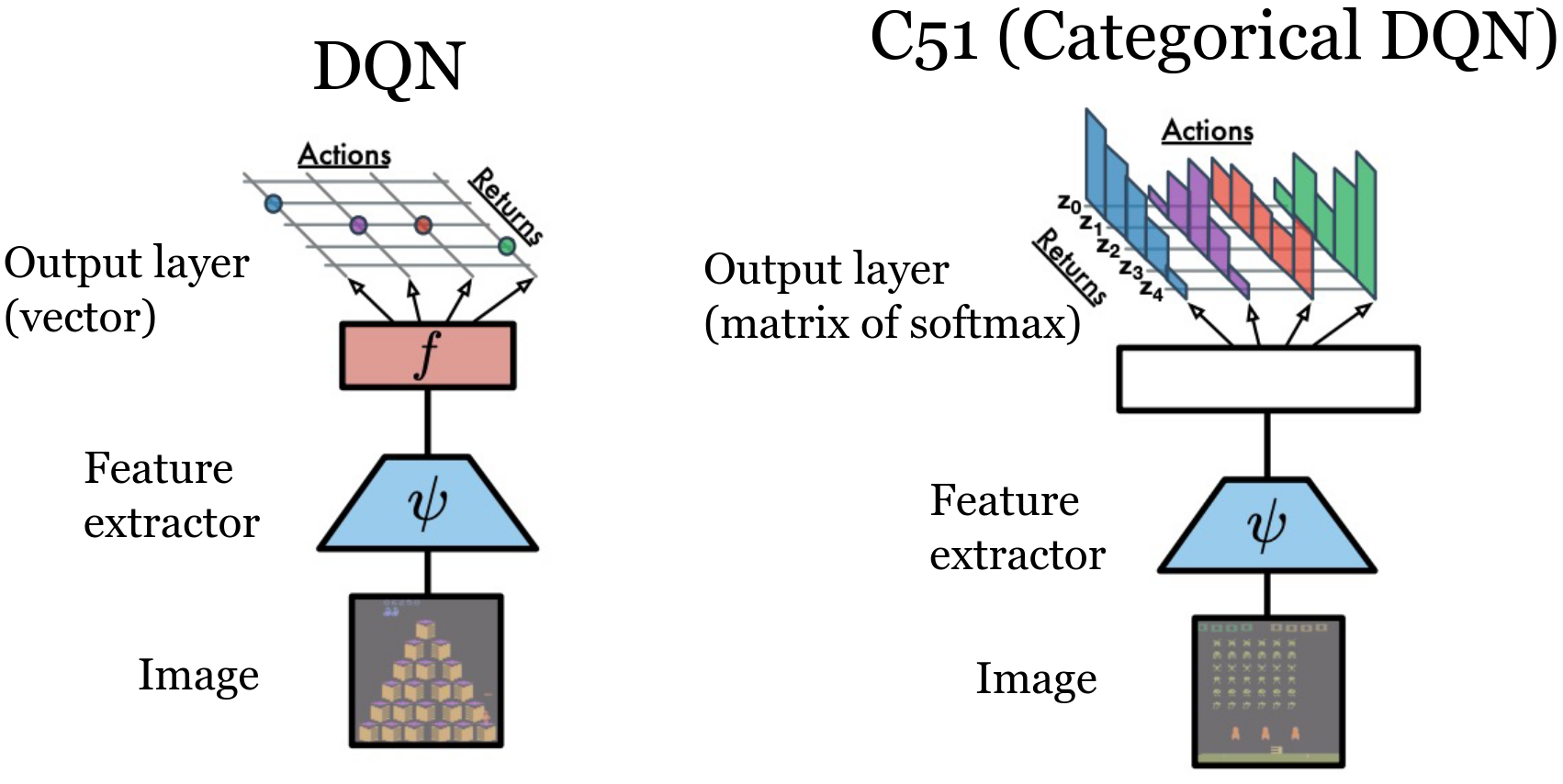
Categorical DQN (C51)
Introduction & Motivation
Classic DQN:
- Learns only the expectation $Q(s,a)=\mathbb{E}[R \mid s,a]$
- Bellman: \(Q(s,a) = R(s,a) + \gamma Q(s', a')\).
- Lost information: variance, skewness, tail (risk) structure.
Distributional RL:
- Model full return random variable \(Z(s,a)\) (not just its mean).
- Distributional Bellman: \(\mathcal{T} Z(s,a) \stackrel{D}{=} R(s,a) + \gamma Z(s', a')\).
- Benefits: richer training signal, more stable gradients, enables risk-sensitive objectives.
Key idea: preserve probabilistic structure throughout the backup,
then take \(\mathbb{E}[Z]\)
only for action selection.
DQN Recap
- Goal: approximate \( Q(s,a) = \mathbb{E}\left[\sum_{t} \gamma^t r_t \mid s,a\right] \)
- Network: input is state, output is vector \( Q(s,a) \) for all actions
- Bellman backup (target): \( y = r + \gamma \max_{a'} Q(s',a') \)
- Loss: mean squared error \( (y - Q(s,a))^2 \)
- Limitation: collapses all uncertainty into a single scalar value
Distributional RL
- Random return: \( Z(s,a) \) is a random variable over \( \mathbb{R} \)
- Distributional Bellman: \( \mathcal{T} Z(s,a) \stackrel{D}{=} r + \gamma Z(S', A') \), i.e., the law is transformed
- Goal: approximate the law of \( Z(s,a) \) (not just \( \mathbb{E}[Z] \))
- Expectation recoverable: \( Q(s,a) = \mathbb{E}[Z(s,a)] \)
- C51: A Distributional Perspective on Reinforcement Learning, Bellemare et al., 2017.
Categorical Approximation (C51)

- Fixed discrete support: \( \{z_i\}_{i=0}^{N-1} \), with \( N = 51 \)
- Bounded interval: \( [V_{\min}, V_{\max}] \)
- \( \Delta z = \frac{V_{\max} - V_{\min}}{N-1} \)
- Network predicts logits \( \to \) softmax \( \to \) \( p_i(s,a) \)
- Approximate distribution: \( \mathbb{P}(Z(s,a) = z_i) = p_i \)
Distributional RL
Example of learned distribution

Distributional RL
Example of learned distribution
Distributional RL
Example of learned distribution
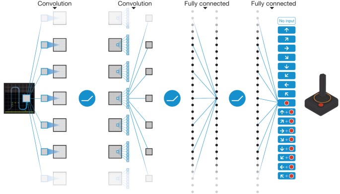
C51 Architecture
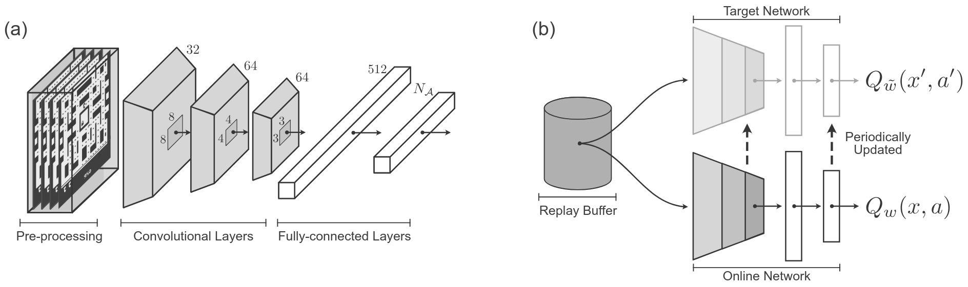
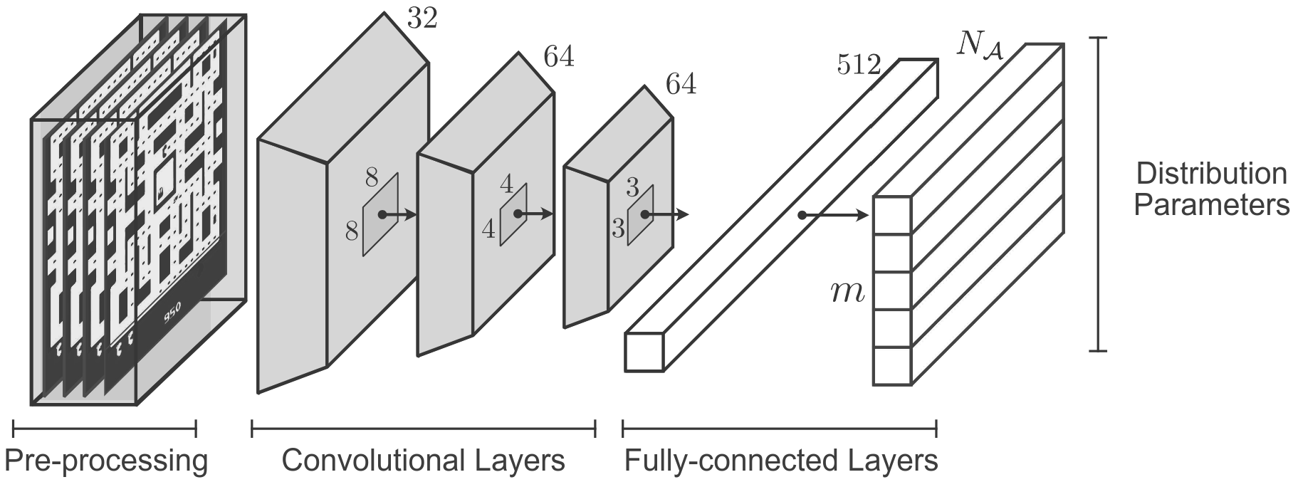
- Backbone identical to DQN: convolutional layers followed by fully connected layers.
- Output: $(\#\text{actions} \times N)$ logits, reshaped to $(\#\text{actions}, N)$.
- Softmax over atoms for each action: $p_i(s,a)$.
- Action selection: $a^* = \arg\max_a \sum_i p_i(s,a) z_i$.
- Target: uses frozen (target) network and projection onto fixed support.
But wait...
Why model the full value distribution if action selection is based only on the expected value?
DQN Algorithm
$\quad\quad$ none
Algorithm parameter:
$\quad\quad$ discount factor $\gamma$
$\quad\quad$ step size $\alpha \in (0,1]$
$\quad\quad$ small $\epsilon > 0$
$\quad\quad$ capacity of the experience replay memory $M$
$\quad\quad$ batch size $m$
$\quad\quad$ target network update frequency $\tau$
Initialize replay memory $\mathcal{D}$ to capacity $M$
Initialize action-value function $\hat{Q}_{\mathbf{\omega_1}}$ with random weights $\mathbf{\omega_1}$
Initialize target action-value function $\hat{Q}_{\mathbf{\omega_2}}$ with weights $\mathbf{\omega_2} = \mathbf{\omega_1}$
FOR EACH episode
$\quad$ $\mathbf{s} \leftarrow \text{env.reset}()$
$\quad$ DO
$\quad\quad$ $\mathbf{a} \leftarrow $$\epsilon\text{-greedy}(\mathbf{s}, \hat{Q}_{\mathbf{\omega_1}})$
$\quad\quad$ $r, \mathbf{s'} \leftarrow \text{env.step}(\mathbf{a})$
$\quad\quad$ Store transition $(\mathbf{s}, \mathbf{a}, r, \mathbf{s'})$ in $\mathcal{D}$
$\quad\quad$ If $\mathcal{D}$ contains "enough" transitions
$\quad\quad\quad$ Sample random batch of transitions $(\mathbf{s}_j, \mathbf{a}_j, r_j, \mathbf{s'}_j)$ from $\mathcal{D}$ with $j=1$ to $m$
$\quad\quad\quad$ For each $j$, set $y_j = \begin{cases} r_j & \text{for terminal } \mathbf{s'}_j\\ r_j + \gamma \max_{\mathbf{a}^\star} \hat{Q}_{\mathbf{\omega_{2}}} (\mathbf{s'}_j)_{\mathbf{a}^\star} & \text{for non-terminal } \mathbf{s'}_j \end{cases}$
$\quad\quad\quad$ Perform a gradient descent step on $\left( y_j - \hat{Q}_{\mathbf{\omega_1}}(\mathbf{s}_j)_{\mathbf{a}_j} \right)^2$ with respect to the weights $\mathbf{\omega_1}$
$\quad\quad\quad$ Every $\tau$ steps reset $\hat{Q}_{\mathbf{\omega_2}}$ to $\hat{Q}_{\mathbf{\omega_1}}$, i.e., set $\mathbf{\omega_2} \leftarrow \mathbf{\omega_1}$
$\quad\quad$ $\mathbf{s} \leftarrow \mathbf{s'}$
$\quad$ UNTIL $\mathbf{s}$ is final
RETURN $\mathbf{\omega_1}$
C51 Algorithm
$\quad$ $\mathbf{s} \leftarrow \text{env.reset}()$
$\quad$ DO
$\quad\quad$ $\mathbf{a} \leftarrow $$\epsilon\text{-greedy}(\mathbf{s}, \hat{Z}_{\mathbf{\omega_1}})$
$\quad\quad$ $r, \mathbf{s'} \leftarrow \text{env.step}(\mathbf{a})$
$\quad\quad$ Store transition $(\mathbf{s}, \mathbf{a}, r, \mathbf{s'})$ in $\mathcal{D}$
$\quad\quad$ IF $\mathcal{D}$ contains "enough" transitions
$\quad\quad\quad$ Sample random batch of transitions $(\mathbf{s}_j, \mathbf{a}_j, r_j, \mathbf{s'}_j)$ from $\mathcal{D}$ with $j=1$ to $m$
$\quad\quad\quad$ FOR EACH transitions $(\mathbf{s}, \mathbf{a}, r, \mathbf{s'})$ of this batch
$\quad\quad\quad\quad$ Apply the Bellman operator
$\quad\quad\quad\quad$ Compute the projection $\Phi$ of $\mathcal{T}^{\pi}Z$ onto the support $\{z_i\}$
$\quad\quad\quad\quad$ Perform a gradient descent step to minimize the cross-entropy
$\quad\quad\quad$ Every $\tau$ steps reset $\hat{Z}_{\mathbf{\omega_2}}$ to $\hat{Z}_{\mathbf{\omega_1}}$, i.e., set $\mathbf{\omega_2} \leftarrow \mathbf{\omega_1}$
$\quad\quad$ $\mathbf{s} \leftarrow \mathbf{s'}$
$\quad$ UNTIL $\mathbf{s}$ is final
RETURN $\mathbf{\omega_1}$
$$Q(s,a) = \mathbb{E}[Z(s,a)] = \sum_i z_i , p_\omega(z_i \mid s,a).$$ The value $Q$ can be obtained as the expectation of $Z$.
Behavior policy: with probability $1-\epsilon$, take the action that maximizes the expected value
according to the current distributional estimate.

Since the support of the target distribution does not necessarily fall exactly on the fixed support of the predicted distribution,
we project it using the operator $(\Phi)$.

Perform a gradient descent step to minimize the cross-entropy between
the predicted distribution and the target distribution.
$$L(\omega) = - \sum_i p_i^{\text{target}} \log p_i^{\text{pred}}$$
C51
Atari Results (Summary)
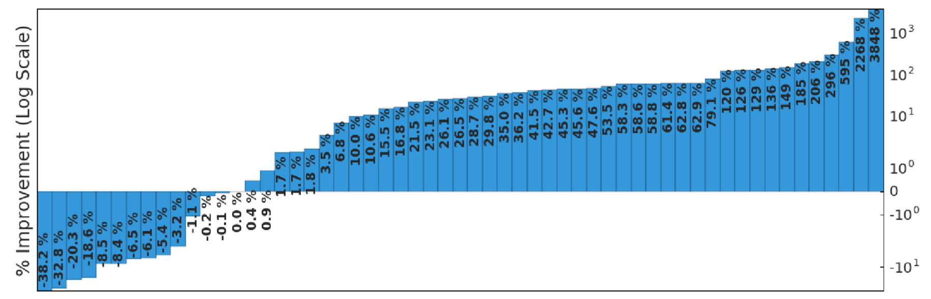
Source: A Distributional Perspective on Reinforcement Learning, Bellemare et al., 2017.
- Improved median score compared to vanilla DQN
- Faster convergence in the first millions of frames
- Reduced training variance
- Foundation for Rainbow (integration of further improvements)
C51
Atari Results (varying number of atoms)
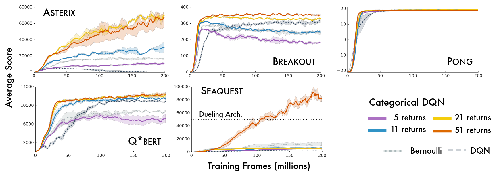
Source: A Distributional Perspective on Reinforcement Learning, Bellemare et al., 2017.
C51
Limitations & Extensions
- Fixed support: risk of saturation if returns fall outside $[V_{\min}, V_{\max}]$
- Uniform resolution: inefficient for modeling sharp tails or skewed distributions
- Extensions:
- QR-DQN: learns quantiles, reducing projection bias
- IQN: continuous implicit quantile function for flexible modeling
- Paradigm: working with distributions enables risk-sensitive and utility-based RL
C51
Conclusion & Discussion
- Moving from expectation to distribution provides a richer learning signal.
- C51 is simple, effective, and forms the basis for many improvements.
- Actions are selected via the expectation: the full distribution is valuable for training and for future risk-sensitive objectives.
- Enables risk-sensitive RL, robustness, and informed exploration.
- Open questions: how to choose the support? How to combine with epistemic uncertainty?
Quantile Regression Deep Q-Network
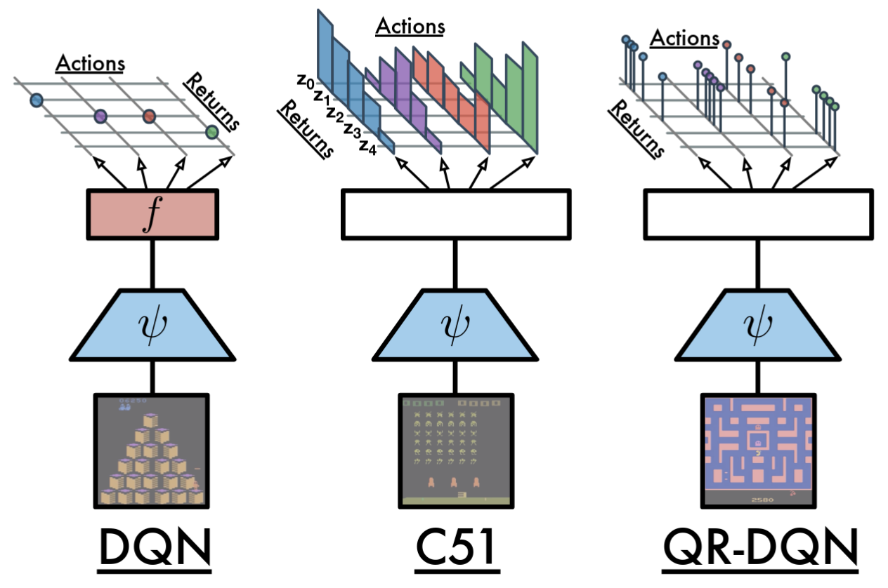
- Represents the value distribution by estimating a fixed set of quantiles.
- Uses quantile regression loss to train the network.
- Improves stability and expressiveness over categorical methods.
Distributional Reinforcement Learning with Quantile Regression, Dabney et al., 2017.
Extensions
QR with Utility / Risk-sensitive RL
- Integrate utility functions into quantile-based RL
for risk-sensitive objectives. - Customize agent behavior: risk-averse, risk-seeking,
or robust policies. - Applications in finance, robotics, and safety-critical domains.
Further Reading
Bellemare, M. G., Dabney, W., & Rowland, M. (2023). Distributional Reinforcement
Learning. MIT Press.
Freely available as an open-access PDF from MIT Press.
Conclusion
- Advanced RL methods address key challenges: exploration, uncertainty, and value modeling.
- Structured exploration (intrinsic rewards, memory, Go-Explore) enables progress in sparse and complex environments.
- Distributional RL provides richer learning signals and opens the door to risk-sensitive and robust agents.
- These advances are foundational for scaling RL to real-world, high-stakes applications.
Perspectives & Open Questions
- How to combine exploration, distributional modeling, and scalability in unified frameworks?
- What are the best strategies for generalization and transfer to new tasks?
- How to ensure safety, robustness, and interpretability in RL agents?
- Other advanced topics: hierarchical RL, meta-learning, large-scale distributed RL, Multi-agent RL.
Key takeaway: Modern RL is a rapidly evolving field—mastering these advanced concepts is crucial for both research and practical applications.